Lecture 24.1

Long-range strain in InGaAs quantum dots — introduction

In the lecture

The plan of Section 24: a numerical experiment on one embedded InAs dot that asks how many atoms are needed before strain and the confined energies stop changing, and how far strain and wavefunctions reach.
How self-assembled dots form (Stranski–Krastanov growth): InAs is 7 % larger than GaAs, and the strained film breaks up into islands that are then capped.
A bulk-like band edge inside a nanometre-sized dot does not exist and cannot be measured; the confined states can be measured optically but are hard to simulate.
Strain moves the energies a lot: in a small InAs pyramid it nearly doubles the local band gap and raises the electron–hole transition energy by about 30 %.
The NEMO 3-D flow: geometry, atomistic (valence force field) relaxation, tight-binding Hamiltonian, single-particle states, then optical and many-body properties.

In this notebook

You compute the strain of a pseudomorphic InAs film with the continuum elasticity solver (opennemo.solvers.elasticity), relax a 7 nm InAs pyramid in GaAs atom by atom with the Keating force field (opennemo.models.mechanics), draw its bond lengths and its "classical" local band edges from strained tight binding (opennemo.models.tb.local_band_edges), compute the electron–hole energy of the same dot with and without strain, and count how many atoms the experiment of the next lectures needs.

Run the notebookEvery number and figure on this page comes from it. Change it, rerun it, take it further.

Download .ipynb View on GitHub

Run it on your own machine

The notebook needs open-nemo (Python ≥ 3.10 and a C++20 compiler; BLAS/LAPACK).

git clone https://github.com/denphi/open-nemo.git && cd open-nemo
python3 -m venv .venv && source .venv/bin/activate
pip install -e ".[notebooks]"
jupyter lab From_Atoms_to_Devices/10_long_range_strain/24_1_long_range_strain_introduction.ipynb

Code17 lines · cell 1

import time

import numpy as np
import matplotlib.pyplot as plt
import opennemo as nemo
from opennemo.models import kp
from opennemo.solvers import elasticity as el
from opennemo.solvers.poisson import Grid
from opennemo.models import kp_grid as kg, mechanics as M
from opennemo.simulations import kp_states as kps
from opennemo.models.tb import local_band_edges
from opennemo.structures.shapes import Box, Dome, Pyramid
from opennemo.structures.structure import Structure
from opennemo.visualization import style

style.use(notebook=True)
T_START = time.time()

1. How do we get quantum dots? Stranski–Krastanov growth#

Self-assembled InAs dots are grown by depositing InAs on a GaAs substrate. The two crystals have the same zincblende structure, but the InAs lattice constant (0.6058 nm) is 7 % larger than that of GaAs (0.5653 nm). The first InAs layer, the wetting layer of about one monolayer, takes the in-plane lattice constant of the substrate: it is squeezed in the plane and, to keep its volume, stretched along the growth direction. Every further layer stores more elastic energy. After a little more than a monolayer the film finds it cheaper to break up into small islands, which can relax by bulging out. Capped with GaAs, the islands become quantum dots: a substrate, a wetting layer, the dot, and a capping layer.

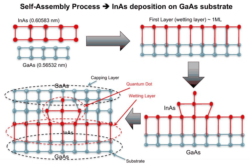Slide 3: Stranski–Krastanov growth of InAs on GaAs Slide 3: InAs (0.60583 nm) on GaAs (0.56532 nm): the first, strained layer (wetting layer), islanding, and the capped dot with its wetting layer, substrate and capping layer.

The lecture lists what such dots carry along from their growth: rough and asymmetric interfaces, strain, and stress-induced (piezoelectric) polarization. The atom positions determine the electronic structure.

For a film that is thin compared with the substrate, the in-plane strain against the film's own lattice is $\varepsilon_\parallel = a_\mathrm{GaAs}/a_\mathrm{InAs} - 1$. With no stress along the growth direction $z$, $\sigma_{zz} = C_{11}\varepsilon_\perp + 2C_{12}\varepsilon_\parallel = 0$ gives $\varepsilon_\perp = -2(C_{12}/C_{11})\,\varepsilon_\parallel$, and the elastic energy per volume is

w = \left(C_{11} + C_{12} - \frac{2C_{12}^2}{C_{11}}\right)\varepsilon_\parallel^2 ,

with $C_{11}$, $C_{12}$ the elastic constants of InAs (GPa). The code evaluates these formulas and checks the energy density with open-nemo's finite-element elasticity solver on a 5 nm InAs film, clamped to a GaAs substrate and periodic in the plane.

Code21 lines · cell 3

GaAs = kp.material("GaAs", temperature=300)            # Vurgaftman et al. (2001), 300 K
InAs = kp.material("InAs", temperature=300)
E0 = GaAs.valence_band_offset                           # energy zero: unstrained GaAs valence-band top


def stiffness(m):
    """Cubic elastic stiffness (GPa, Voigt) of a k·p material."""
    return el.cubic_stiffness(m.c11, m.c12, m.c44)


def misfit(m):
    """Eigenstrain of m on the GaAs reference lattice: a_m / a_GaAs - 1."""
    return m.lattice_constant / GaAs.lattice_constant - 1


for m in (GaAs, InAs):
    print(f"{m.name}: a = {m.lattice_constant:.5f} nm, E_g = {m.band_gap:.3f} eV, "
          f"E_c = {m.valence_band_offset + m.band_gap - E0:+.3f} eV, "
          f"E_v = {m.valence_band_offset - E0:+.3f} eV, "
          f"a_c = {m.ac:+.2f} eV, m_e = {m.electron_mass:.3f} m0")
print(f"InAs misfit on GaAs: {100 * misfit(InAs):.2f} %")

GaAs: a = 0.56532 nm, E_g = 1.422 eV, E_c = +1.422 eV, E_v = +0.000 eV, a_c = -7.17 eV, m_e = 0.067 m0
InAs: a = 0.60583 nm, E_g = 0.354 eV, E_c = +0.564 eV, E_v = +0.210 eV, a_c = -5.08 eV, m_e = 0.026 m0
InAs misfit on GaAs: 7.16 %

Code23 lines · cell 4

eps_par = GaAs.lattice_constant / InAs.lattice_constant - 1
eps_perp = -2 * InAs.c12 / InAs.c11 * eps_par
w = (InAs.c11 + InAs.c12 - 2 * InAs.c12**2 / InAs.c11) * eps_par**2 * el.GPA_NM3_TO_EV   # eV / nm^3
a_perp = InAs.lattice_constant * (1 + eps_perp)
v_pair = GaAs.lattice_constant**2 * a_perp / 4                                       # nm^3 per InAs pair
print(f"pseudomorphic InAs on GaAs: eps_par = {100 * eps_par:.2f} %, eps_perp = {100 * eps_perp:+.2f} %, "
      f"a_perp = {a_perp:.4f} nm")
print(f"elastic energy: {w:.3f} eV/nm^3 = {1e3 * w * v_pair:.0f} meV per InAs pair, "
      f"{w * a_perp / 2:.2f} eV per nm^2 for each added monolayer")

# the same film with finite elements: GaAs substrate (z < 5 nm, bottom clamped) and 5 nm of InAs
film = el.Elasticity.from_regions(
    Grid(np.linspace(0, 1, 3), np.linspace(0, 1, 3), np.linspace(0, 10, 41)),
    [(None, stiffness(GaAs), 0.0), (Box((-1, -1, 5), (2, 2, 11)), stiffness(InAs), misfit(InAs))],
    periodic=(True, True, False))
film.fix(np.isclose(film.grid.nodes[:, 2], 0.0))
film_result = film.solve()
eps_film = film_result.local_strain_in("biot")[-1]                  # a cell of the film, against InAs
w_gaas = (InAs.c11 + InAs.c12 - 2 * InAs.c12**2 / InAs.c11) * misfit(InAs) ** 2 * el.GPA_NM3_TO_EV
print(f"finite elements: eps_par = {100 * eps_film[0, 0]:.2f} %, eps_perp = {100 * eps_film[2, 2]:+.2f} %; "
      f"energy {film_result.energy / 5.0:.3f} eV/nm^3 of film")
print(f"the formula with the strain measured from the GaAs lattice (eps_par = -{100 * misfit(InAs):.2f} %): "
      f"{w_gaas:.3f} eV/nm^3")

pseudomorphic InAs on GaAs: eps_par = -6.69 %, eps_perp = +7.27 %, a_perp = 0.6499 nm
elastic energy: 2.214 eV/nm^3 = 115 meV per InAs pair, 0.72 eV per nm^2 for each added monolayer
finite elements: eps_par = -6.69 %, eps_perp = +7.27 %; energy 2.543 eV/nm^3 of film
the formula with the strain measured from the GaAs lattice (eps_par = -7.16 %): 2.543 eV/nm^3

The solver reproduces the strains of the formula. Its energy is 15 % higher, and the last line shows why: the solver is linear elasticity about the GaAs lattice, in which the film is squeezed by the full misfit of 7.16 %, while the formula above measured the squeeze from the InAs lattice (6.69 %). At strains of 7 % linear elasticity is not unique to better than this. Either way, each InAs pair in the film stores more than 0.1 eV of elastic energy, and every added monolayer adds the same amount again: the energy grows linearly with the thickness, while the energy an island gains by relaxing at its free surfaces does not. That is why the film breaks up into dots after a monolayer or two, and why these dots, once capped, sit in a crystal that is strained around them over long distances, the subject of this section.

2. Strain effects are very critical: a small InAs pyramid#

The lecture illustrates the size of the effect with a small toy dot: an InAs pyramid of 7 nm × 7 nm base and 3 nm height embedded in GaAs. Mechanically, the atoms move to minimize the elastic energy of a valence force field (Keating's model: bond-stretching and bond-bending springs), so bond lengths and bond angles change. Electronically, the overlap of the orbitals on neighbouring atoms changes with the bond vector $\mathbf R_{ij}$, and with it the band gaps and the effective masses. An atomistic tight-binding model captures this directly.

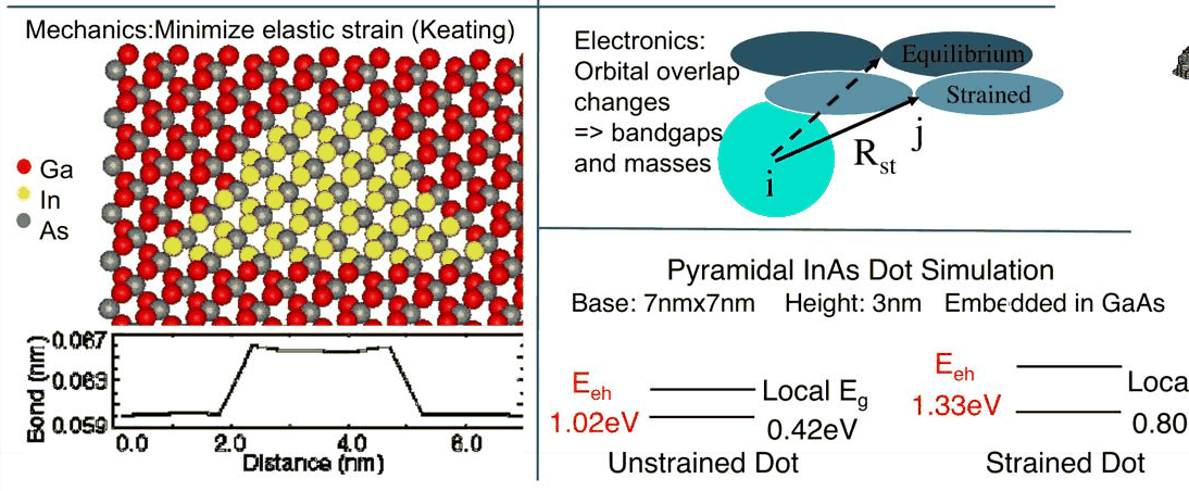Slide 5: atomistic relaxation and the strain shift of a pyramidal InAs dot Slide 5: a cut through the relaxed pyramid (Ga red, In yellow, As grey), the bond length along a line through it, and the energies of the unstrained and strained dot: local gap 0.42 → 0.80 eV, electron–hole energy 1.02 → 1.33 eV.

The structure below is the lecture's toy: the pyramid (base 7 nm, height 3 nm, no wetting layer) in a periodic GaAs box of 20 × 20 × 16 conventional cells (11.3 × 11.3 × 9.0 nm³) held at the GaAs lattice constant, relaxed with Keating's force field (Martin's parameters) by the FIRE minimizer.

Code22 lines · cell 6

tb_set = nemo.structures.materials.load("klimeck2002_sp3d5s")       # NEMO 3-D's sp3d5s* parameters
G_tb, I_tb = tb_set["GaAs"], tb_set["InAs"]
lat = nemo.structures.lattice.from_material(G_tb)
a = G_tb.lattice_constant
NX, NZ = 20, 16
cell, basis, sub = lat.conventional, lat.conventional_basis, lat.conventional_sublattice
grid_idx = np.stack(np.meshgrid(np.arange(NX), np.arange(NX), np.arange(NZ), indexing="ij"), -1)
grid_idx = grid_idx.reshape(-1, 3)
pos = ((grid_idx @ cell)[:, None, :] + basis[None]).reshape(-1, 3)
sublattice = np.tile(sub, len(grid_idx))
species = np.array([lat.species[i] for i in sublattice], dtype=object)
L, LZ, Z0 = NX * a, NZ * a, 6 * a                                      # box (nm), pyramid base height
pyramid = Pyramid((L / 2 - 3.5, L / 2 - 3.5, Z0), (7.0, 7.0), 3.0)
species[(species == "Ga") & pyramid.contains(pos)] = "In"
crystal = Structure(pos, list(species), np.diag([L, L, LZ]), sublattice, lat)

t0 = time.time()
relaxed = M.relax(M.Keating(crystal), tol=1e-4, method="fire")
t_relax = time.time() - t0
x = relaxed["positions"]
print(f"{crystal.num_atoms} atoms ({np.sum(species == 'In')} In); relaxed in {relaxed['iterations']} FIRE "
      f"steps, {t_relax:.1f} s (max force {relaxed['max_force']:.1e} eV/nm)")

51200 atoms (1082 In); relaxed in 242 FIRE steps, 0.7 s (max force 7.5e-05 eV/nm)

Two views of the relaxed crystal follow, both on the line of cations along $x$ through the pyramid's axis, 1 nm above its base:

the mean length of each cation's four bonds (the quantity of the slide's bond-length plot);
the "classical" local band edges: for each cation, open-nemo builds a bulk crystal from its four actual bonds, repeated periodically, and diagonalizes NEMO 3-D's strained $sp^3d^5s^*$ tight-binding Hamiltonian at $\Gamma$ (Klimeck et al., CMES 2002). Lecture 24.2 uses the same construction.

The dashed lines are the band edges of unstrained bulk InAs and GaAs from the same parameters.

Code39 lines · cell 8

from scipy.spatial import cKDTree

box = np.array([L, L, LZ])
cations = np.flatnonzero(species != "As")
anions = np.flatnonzero(species == "As")
wrap = lambda p: np.mod(np.mod(p, box), box)                         # into [0, box)
dist, _ = cKDTree(wrap(x[anions]), boxsize=box).query(wrap(x[cations]), k=4)
bond = np.full(len(species), np.nan)
bond[cations] = dist.mean(axis=1)                                    # nm, mean of each cation's four bonds

zc, yc = x[cations, 2], x[cations, 1]
z_line = zc[np.argmin(np.abs(zc - (Z0 + 1.0)))]
y_line = yc[np.argmin(np.abs(yc - L / 2))]
on_line = (np.abs(zc - z_line) < 0.02) & (np.abs(yc - y_line) < 0.02)
line = cations[on_line][np.argsort(x[cations[on_line], 0])]
x_line = x[line, 0] - L / 2
in_dot = species[line] == "In"

both = nemo.structures.materials.alloy(G_tb, I_tb)
t0 = time.time()
tb_edges = local_band_edges(both, crystal, positions=x, atoms=line)
t_edges = time.time() - t0
bulk = {}
for name, mat in (("GaAs", G_tb), ("InAs", I_tb)):
    lat_m = nemo.structures.lattice.from_material(mat)
    g1 = np.stack(np.meshgrid(*(np.arange(2),) * 3, indexing="ij"), -1).reshape(-1, 3)
    p1 = ((g1 @ lat_m.conventional)[:, None, :] + lat_m.conventional_basis[None]).reshape(-1, 3)
    s1 = np.tile(lat_m.conventional_sublattice, len(g1))
    sp1 = [lat_m.species[i] for i in s1]
    bulk_s = Structure(p1, sp1, 2 * lat_m.conventional, s1, lat_m)
    e = local_band_edges(both, bulk_s, atoms=[sp1.index(name[:2])])          # one cation
    bulk[name] = (e["conduction"][0], e["heavy_hole"][0])
gap = tb_edges["conduction"] - np.maximum(tb_edges["heavy_hole"], tb_edges["light_hole"])
print(f"unstrained bulk gaps: GaAs {bulk['GaAs'][0] - bulk['GaAs'][1]:.3f} eV, "
      f"InAs {bulk['InAs'][0] - bulk['InAs'][1]:.3f} eV")
print(f"mean bond length on the line: GaAs at its end {bond[line][0]:.4f} nm, inside the dot "
      f"{bond[line][in_dot].mean():.4f} nm (unstrained InAs {np.sqrt(3) / 4 * I_tb.lattice_constant:.4f} nm)")
print(f"strained local gap in the dot: {gap[in_dot].min():.3f} to {gap[in_dot].max():.3f} eV, "
      f"mean {gap[in_dot].mean():.3f} eV ({t_edges:.1f} s for {len(line)} cations)")

unstrained bulk gaps: GaAs 1.424 eV, InAs 0.370 eV
mean bond length on the line: GaAs at its end 0.2447 nm, inside the dot 0.2547 nm (unstrained InAs 0.2623 nm)
strained local gap in the dot: 0.656 to 0.917 eV, mean 0.839 eV (0.3 s for 18 cations)

Code17 lines · cell 9

fig, (ax1, ax2) = plt.subplots(1, 2, figsize=(11, 3.8))
ax1.plot(x_line, bond[line], marker="o", ms=3, **style.series())
ax1.axhline(np.sqrt(3) / 4 * G_tb.lattice_constant, **style.series("context", label="bulk GaAs"))
ax1.axhline(np.sqrt(3) / 4 * I_tb.lattice_constant, **style.series("context", ls="--", label="bulk InAs"))
ax1.set(xlabel="x (nm), through the pyramid axis", ylabel="mean bond length (nm)",
        title="bond length 1 nm above the base")
ax1.legend(frameon=False, fontsize=8)
labels = (("conduction", "$E_c$"), ("heavy_hole", "$E_{HH}$"), ("light_hole", "$E_{LH}$"))
for i, (key, lab) in enumerate(labels):
    ax2.plot(x_line, tb_edges[key], "o-", ms=3, color=style.sweep(3)[i], label=lab)
for name, ls in (("GaAs", ":"), ("InAs", "--")):
    for e in bulk[name]:
        ax2.axhline(e, **style.series("context", ls=ls))
ax2.set(xlabel="x (nm), through the pyramid axis", ylabel="local band edge (eV)",
        title="local band edges (strained sp3d5s*)")
ax2.legend(frameon=False, fontsize=8, ncol=3)
fig.tight_layout()

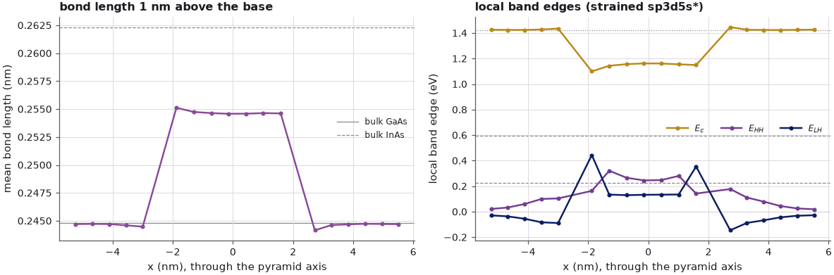
Figure computed by the notebook with open-nemo

Inside the pyramid the bonds are 0.255 nm long, between the GaAs (0.245 nm) and the bulk InAs (0.262 nm) values: the InAs is squeezed by the surrounding GaAs, and the GaAs next to it is stretched. The local band gap of the squeezed InAs is more than twice its bulk value (0.37 eV in this parameter set, 0.42 eV on the slide): 0.84 eV on average, 0.80 eV on the slide. It is also not a flat profile: the gap varies by 0.26 eV across the dot, and the band edges are shaped by the strain field, with heavy and light holes split differently at the centre and at the edges.

How much does this matter for what is measured, the electron–hole transition energy? Answering that needs the confined states. The tight-binding states of this crystal are a sparse eigenproblem of half a million orbitals; we take the continuum route instead, the one the rest of the section uses to reach much larger domains:

strain from finite-element elasticity (el.Elasticity): each material is stress-free at its own lattice constant (its eigenstrain against the GaAs reference lattice), with cubic elastic constants;
local band edges from the strain at each point: the zone-centre eigenvalues of the 8-band k·p Hamiltonian with its Bir–Pikus deformation potentials (kp.bulk_hamiltonian(..., strain=)), the continuum analogue of the tight-binding local band edges above;
confined levels: here, for a dot this small, the full 8-band k·p Hamiltonian on a 0.5 nm grid (kp_grid.KPGrid with the strain field, kp_states.electrons / holes); in Lectures 24.2–24.4, a single-band effective-mass Hamiltonian on the local band edges, cheap enough for 100 nm domains.

Its parameters (Vurgaftman et al. 2001, 300 K) give InAs a gap of 0.354 eV, so absolute energies differ from the lecture's tight binding by tens of meV; the strain effects are what we compare. The function below computes the local band edges; the check compares it with a direct diagonalization.

Code44 lines · cell 11

VOIGT = [(0, 0), (1, 1), (2, 2), (1, 2), (0, 2), (0, 1)]
_LINEAR = {}


def local_edges(m, eps):
    """Local band edges (eV, from E0) of material m under the strains eps (n, 3, 3): the zone-centre
    eigenvalues of its 8-band k·p Hamiltonian (Bir-Pikus strain terms). Returns E_c, E_HH, E_LH; the
    heavy holes are the valence pair with the least |Z> character (z: growth axis)."""
    if m.name not in _LINEAR:                            # H(eps) = H0 + sum eps_ij D_ij: linear in eps
        h0 = kp.bulk_hamiltonian(m, np.zeros(3), 8)
        d = []
        for i, j in VOIGT:
            u = np.zeros((3, 3))
            u[i, j] = u[j, i] = 1.0
            d.append(kp.bulk_hamiltonian(m, np.zeros(3), 8, strain=u) - h0)
        _LINEAR[m.name] = h0, np.array(d)
    h0, d = _LINEAR[m.name]
    v = np.stack([eps[:, i, j] for i, j in VOIGT], -1)
    w, u = np.linalg.eigh(h0[None] + np.einsum("na,aij->nij", v, d))
    z = np.abs(u[:, 3, 2:6]) ** 2 + np.abs(u[:, 7, 2:6]) ** 2   # basis S, X, Y, Z per spin
    order = np.argsort(z, axis=1)
    top = w[:, 2:6]
    e_hh = np.take_along_axis(top, order[:, :2], 1).max(1)
    e_lh = np.take_along_axis(top, order[:, 2:], 1).max(1)
    return w[:, 6] - E0, e_hh - E0, e_lh - E0


def region_at(result, points):
    """Region index (0: the GaAs matrix, >0: the dot) of the finite-element cell containing each
    point: the cell whose material local_strain_at measures the strain against."""
    p = result.problem
    ids = []
    for d, a in enumerate(p.grid.axes):
        x = points[:, d]
        if p.periodic[d]:
            x = a[0] + np.mod(x - a[0], a[-1] - a[0])
        ids.append(np.clip(np.searchsorted(a, x, side="right") - 1, 0, len(a) - 2))
    return p.material[np.ravel_multi_index(tuple(ids), p.cell_shape)]


eps_test = np.array([[-0.05, 0.01, 0.0], [0.01, -0.05, 0.0], [0.0, 0.0, 0.04]])
direct = np.linalg.eigvalsh(kp.bulk_hamiltonian(InAs, np.zeros(3), 8, strain=eps_test)) - E0
print("direct 8-band:  E_c, top valence =", np.round(direct[[6, 5]], 5))
print("local_edges:    E_c, E_HH, E_LH  =", np.round(np.ravel(local_edges(InAs, eps_test[None])), 5))

direct 8-band:  E_c, top valence = [0.86859 0.32936]
local_edges:    E_c, E_HH, E_LH  = [0.86859 0.32936 0.1134 ]

Code31 lines · cell 12

# the same pyramid in the same periodic GaAs box, by finite elements
t0 = time.time()
nx, nz = 36, 29                                                      # about 0.31 nm per cell
toy = el.Elasticity.from_regions(
    Grid(np.linspace(0, L, nx + 1), np.linspace(0, L, nx + 1), np.linspace(0, LZ, nz + 1)),
    [(None, stiffness(GaAs), 0.0), (pyramid, stiffness(InAs), misfit(InAs))], periodic=(True, True, True))
toy_strain = toy.solve()
t_fem = time.time() - t0

# 8-band k·p levels on a 10.5 x 10.5 x 7.5 nm crop around the dot (hard walls), without and with
# strain; the 0.5 nm grid is placed so that no point lies on a face of the pyramid
t0 = time.time()
crop = np.array([10.5, 10.5, 7.5])
origin = np.array([L / 2 - 5.25, L / 2 - 5.25, Z0 - 2.75])
in_pyramid = lambda p: region_at(toy_strain, p + origin) > 0          # the cells' material
probe = kg.KPGrid.from_shapes(crop, 0.5, [GaAs, InAs], [(in_pyramid, 1)])
toy_levels = {}
for label, eps in (("unstrained", None), ("strained", toy_strain.local_strain_at(probe.positions + origin))):
    g = kg.KPGrid.from_shapes(crop, 0.5, [GaAs, InAs], [(in_pyramid, 1)], strain=eps)
    toy_levels[label] = (kps.electrons(g, 1).energies[0] - E0, kps.holes(g, 1).energies[-1] - E0)
t_levels = time.time() - t0
centre = np.array([[L / 2, L / 2, Z0 + 1.0]])
for label, (e1, h1) in toy_levels.items():
    eps_c = np.zeros((1, 3, 3)) if label == "unstrained" else toy_strain.local_strain_at(centre)
    ec, hh, lh = local_edges(InAs, eps_c)
    print(f"{label:10s}: local gap 1 nm above the base {ec[0] - max(hh[0], lh[0]):.3f} eV; e1 = {e1:.3f} eV, "
          f"h1 = {h1:+.3f} eV, E_eh = e1 - h1 = {e1 - h1:.3f} eV")
e_eh = {k: v[0] - v[1] for k, v in toy_levels.items()}
print(f"strain raises the transition energy by {1e3 * (e_eh['strained'] - e_eh['unstrained']):.0f} meV, "
      f"{100 * (e_eh['strained'] / e_eh['unstrained'] - 1):.0f} % ({probe.num_points} grid points x 8 bands; "
      f"finite elements {t_fem:.1f} s, levels {t_levels:.1f} s)")

unstrained: local gap 1 nm above the base 0.354 eV; e1 = 1.220 eV, h1 = +0.058 eV, E_eh = e1 - h1 = 1.162 eV
strained  : local gap 1 nm above the base 0.879 eV; e1 = 1.485 eV, h1 = +0.095 eV, E_eh = e1 - h1 = 1.391 eV
strain raises the transition energy by 229 meV, 20 % (5600 grid points x 8 bands; finite elements 0.2 s, levels 8.1 s)

The continuum model tells the same story as the slide, a little more weakly. Without strain the 8-band model puts the electron–hole energy at 1.16 eV (1.02 eV on the slide); with strain the local gap at the dot's centre more than doubles, the electron is pushed up, and the transition energy rises by about 230 meV, 20 % (310 meV, 30 % on the slide with tight binding). The single-band models of the next lectures would be cruder still for a dot this small, whose electron sits a few hundred meV above the InAs band edge where the conduction band is far from parabolic. The conclusion is the lecture's: a model without strain is not a little off; it is wrong by a couple of hundred meV.

The lecture's second point is the other half of the title: these strain fields are very far reaching. That is what makes the dots hard to simulate.

3. The computational flow of NEMO 3-D#

Slide 6: the computational flow of NEMO 3-D 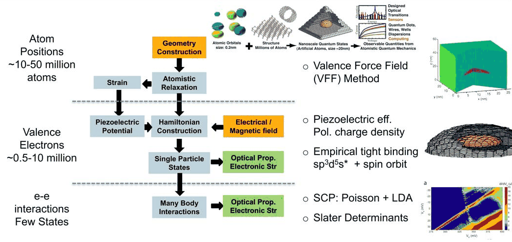Slide 6: NEMO 3-D's multi-scale flow: geometry, atomistic relaxation (valence force field, 10–50 million atoms), Hamiltonian construction (empirical $sp^3d^5s^*$ tight binding with spin–orbit, 0.5–10 million atoms), single-particle states, then many-body interactions for a few states.

The flow has three levels. Atom positions are found for tens of millions of atoms by minimizing a valence force field; the strain field and its piezoelectric potential follow from them. The valence electrons are then described by an empirical tight-binding Hamiltonian on 0.5–10 million atoms, which gives the single-particle states and their optical properties (electric and magnetic fields enter the Hamiltonian). Finally, a few of those states are used for many-body calculations: self-consistent Poisson plus local-density approximation, or configuration interaction with Slater determinants.

Each step has its open-nemo counterpart, and §2 has just run the first ones:

NEMO 3-D step	open-nemo	in §2
geometry construction	`Structure`, `structures.shapes`	51,200 atoms, pyramid
atomistic relaxation (VFF)	`mechanics.Keating`, `mechanics.relax`	FIRE relaxation
strain	`mechanics.atomic_strain`; continuum `solvers.elasticity`	bonds, finite elements
Hamiltonian construction	`models.tb.SlaterKoster(..., strain="bond_length")`	local band edges
single-particle states	`nemo.eigenstates`	effective-mass levels
piezoelectric potential	`simulations.piezoelectric`	(not here)
many-body interactions	`simulations.configuration_interaction`	(not here)

Code5 lines · cell 14

for step, sec in (("atomistic relaxation, 51,200 atoms", t_relax),
                  (f"tight-binding local band edges, {len(line)} cations", t_edges),
                  (f"finite-element strain, {toy.num_cells} cells", t_fem),
                  ("8-band k·p levels, unstrained and strained", t_levels)):
    print(f"{step:45s} {sec:6.1f} s")

atomistic relaxation, 51,200 atoms               0.7 s
tight-binding local band edges, 18 cations       0.3 s
finite-element strain, 37584 cells               0.2 s
8-band k·p levels, unstrained and strained       8.1 s

At this size every step takes seconds. The atomistic electronic-structure step is the expensive one: it grows with the number of atoms in the electronic domain, and for the realistic dots of the next lectures that domain holds millions of atoms.

4. How many atoms is enough?#

The numerical experiment of this section is built on a larger dot: a dome of 30 nm diameter and 5 nm height, embedded in GaAs. Its physical structure is an ordered crystal; relaxing the strain moves the atoms slightly; the electronic structure is then computed for the atoms held fixed, giving eigenenergies and eigenstates; classical local band-edge diagrams help to interpret them. The lecture asks four questions:

How many atoms are needed before the strain converges?
How far does the strain reach?
How many atoms are needed before the eigenenergies converge?
How far does the electronic wavefunction reach?

A GaAs crystal holds 8 atoms per cubic cell of side $a = 0.56532$ nm, 44.2 atoms per nm³. A box that extends a buffer $b$ beyond the dot in every direction, $(30 + 2b)^2 (5 + 2b)$ nm³, holds:

Code17 lines · cell 16

a_gaas = 0.56532                                                    # nm, the value on the slides
density = 8 / a_gaas**3                                             # atoms per nm^3
buffers = np.arange(0, 41)
atoms = density * (30 + 2 * buffers) ** 2 * (5 + 2 * buffers)
for b in (4, 12, 20, 24, 40):
    n_b = density * (30 + 2 * b) ** 2 * (5 + 2 * b) / 1e6
    print(f"buffer {b:2d} nm: box {30 + 2 * b} x {30 + 2 * b} x {5 + 2 * b} nm^3, {n_b:6.2f} million atoms")
fig, ax = plt.subplots(figsize=(6.5, 3.6))
ax.semilogy(buffers, atoms / 1e6, **style.series())
marks = ((4, "electronic domain (24.3)"), (20, "year-2000 electronic limit"), (24, "strain domain (24.3)"))
for b, lab in marks:
    n = density * (30 + 2 * b) ** 2 * (5 + 2 * b) / 1e6
    ax.plot(b, n, "o", color=style.OPEN_NEMO)
    ax.annotate(f"{n:.2f} M: {lab}", (b, n), xytext=(5, -12), textcoords="offset points", fontsize=8)
ax.set(xlabel="GaAs buffer around the dot, b (nm)", ylabel="atoms (millions)",
       title="atoms in a box around a 30 nm x 5 nm dot")
fig.tight_layout()

buffer  4 nm: box 38 x 38 x 13 nm^3,   0.83 million atoms
buffer 12 nm: box 54 x 54 x 29 nm^3,   3.74 million atoms
buffer 20 nm: box 70 x 70 x 45 nm^3,   9.76 million atoms
buffer 24 nm: box 78 x 78 x 53 nm^3,  14.28 million atoms
buffer 40 nm: box 110 x 110 x 85 nm^3,  45.54 million atoms

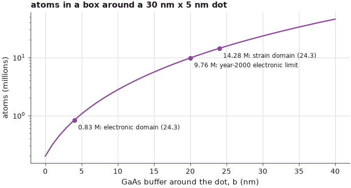
The count grows with the cube of the buffer: 0.83 million atoms for a 4 nm buffer, 9.76 million for the 20 nm buffer that was the limit of electronic-structure calculations in 2000, 14.3 million for 24 nm. The experiment of Lectures 24.2 and 24.3 lives between these numbers.

A first look at why the buffer has to be large: the strain field of this dot (pure InAs, free outer surfaces as in the lecture's first experiment, 20 nm of GaAs around it), from the finite-element solver, along the vertical axis through the dot and along a lateral line at half its height.

Code38 lines · cell 18

def graded(lo, hi, core_lo, core_hi, h, h_max=2.0, growth=1.25):
    """Nodes from lo to hi: spacing h on the core, growing by `growth` per cell outside it."""
    out = list(np.arange(core_lo, core_hi + 1e-9, h))
    for end, sign in ((hi, 1), (lo, -1)):
        s, xx = h, out[-1] if sign > 0 else out[0]
        while True:
            s = min(s * growth, h_max)
            xx += sign * s
            if (xx >= end - 0.3 * s) if sign > 0 else (xx <= end + 0.3 * s):
                break
            out = out + [xx] if sign > 0 else [xx] + out
        out = out + [end] if sign > 0 else [end] + out
    return np.array(out)


R, H, B = 15.0, 5.0, 20.0
dome = Dome((0, 0, 0), (R, R, H))
xa, za = graded(-R - B, R + B, -R - 1, R + 1, 1.0), graded(-B, H + B, -1, H + 1, 0.5)
t0 = time.time()
big = el.Elasticity.from_regions(Grid(xa, xa, za), [(None, stiffness(GaAs), 0.0),
                                                     (dome, stiffness(InAs), misfit(InAs))]).solve()
print(f"{len(xa)} x {len(xa)} x {len(za)} nodes, {time.time() - t0:.1f} s")
s_up = np.linspace(0.05, B - 0.05, 200)                             # distance from the dot's surface
cuts = {"vertical (above the apex)": np.c_[0 * s_up, 0 * s_up, H + s_up],
        "vertical (below the base)": np.c_[0 * s_up, 0 * s_up, -s_up],
        "lateral (at half height)": np.c_[R * np.sqrt(1 - 0.25) + s_up, 0 * s_up, H / 2 + 0 * s_up]}
fig, ax = plt.subplots(figsize=(6.5, 3.8))
for (lab, pts), col in zip(cuts.items(), style.sweep(3)):
    e = big.local_strain_at(pts)
    mag = np.sqrt(np.einsum("nij,nij->n", e, e))                      # |eps|, Frobenius norm
    ax.semilogy(s_up, mag, color=col, label=lab)
    print(f"{lab:27s}: |eps| = {100 * mag[0]:.2f} % at the surface, {100 * np.interp(10, s_up, mag):.3f} % "
          f"at 10 nm, {100 * np.interp(19, s_up, mag):.3f} % at 19 nm")
ax.set(xlabel="distance from the dot's surface (nm)", ylabel="|ε| in the GaAs",
       title="strain around a 30 nm InAs dome")
ax.legend(frameon=False, fontsize=8)
fig.tight_layout()
print(f"notebook run time: {time.time() - T_START:.0f} s")

53 x 53 x 39 nodes, 0.8 s
vertical (above the apex)  : |eps| = 2.53 % at the surface, 1.216 % at 10 nm, 0.604 % at 19 nm
vertical (below the base)  : |eps| = 2.15 % at the surface, 1.236 % at 10 nm, 0.754 % at 19 nm
lateral (at half height)   : |eps| = 6.31 % at the surface, 0.400 % at 10 nm, 0.076 % at 19 nm
notebook run time: 11 s

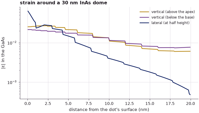
The strain in the GaAs is 2–6 % at the dot's surface (the steps are the finite-element cells, constant strain each, which grow away from the dot). Ten nanometres away it is still 0.4 % at the side of the dot and 1.2 % above and below it; at the outer surface of the box, 20 nm from the dot, it has fallen below 0.1 % laterally but not below 0.6 % vertically: the flat dot pushes the whole crystal apart along $z$. A strain of 0.5 % moves the GaAs conduction band by about $a_c \operatorname{tr}\varepsilon$, a few tens of meV, comparable to the energies a dot calculation must resolve. The next three lectures turn these observations into answers: expanding the strain domain (24.2), shrinking the electronic domain (24.3), and choosing the boundary conditions (24.4).

Summary#

Self-assembled InAs dots form because InAs is 7.2 % larger than GaAs: a pseudomorphic InAs film stores more than 0.1 eV per InAs pair, a cost that grows linearly with the film thickness until the film islands.
A bulk band edge inside a dot is a concept, not a measurable quantity; the confined states are what experiments see.
Strain is decisive: in a 7 nm InAs pyramid it more than doubles the local gap (0.37 → 0.84 eV in tight binding) and raises the electron–hole energy by about 230 meV in 8-band k·p (310 meV on the slide).
NEMO 3-D's flow (geometry, VFF relaxation, tight binding, states, many-body) maps one-to-one onto open-nemo functions.
A 30 nm dot with a 20 nm buffer means about 10 million atoms; the strain around it is still 0.4–1.2 % 10 nm away from the dot, and decays most slowly along the growth direction.

Exercises#

Make the pyramid of §2 taller (4 nm), or rerun its 8-band levels at a grid spacing of 0.4 nm. How do the strained local gap and $E_{eh}$ change, and how much of the change at 0.4 nm is the grid?
Repeat the film calculation of §1 for In${0.3}$Ga${0.7}$As on GaAs (kp.material("InGaAs", x=0.3, temperature=300)) and for InAs on InP (kp.material("InP")). How much less elastic energy per pair does each film store, and what does that suggest about the thickness at which it islands?
In §4, clamp the bottom face of the box (fix the nodes at $z = -20$ nm) and redraw the strain decay. Which of the three cuts changes most?